
Walk forward validation is the process of repeatedly optimizing a model or strategy on a fixed in-sample window, then evaluating it on the immediately following out-of-sample period, rolling that window forward until the full dataset is consumed. It gives you an honest, out-of-time performance estimate that a single backtest cannot provide. If you're building any time-series model or trading strategy that will be retrained or re-parameterized over time, walk-forward is the right validation framework to use.
Three anchors worth knowing before you go further:
- Robert E. Pardo formalized Walk-Forward Analysis in his foundational work on strategy testing, establishing the iterative IS/OOS loop that practitioners still use today.
- scikit-learn's TimeSeriesSplit provides a code-level entry point for time-aware splitting, though it lacks finance-specific purging and embargo logic out of the box.
- Trade-4 offers a no-code backtesting platform built for small-cap traders where you can configure IS/OOS windows, cost models, and multi-run grids without managing a local database.
Key Takeaways
Walk-forward validation is reliable only when IS optimization, OOS evaluation, cost modeling, and multiple-testing correction are all applied together across enough folds to generate statistically meaningful trade counts.
| Point | Details |
|---|---|
| IS/OOS loop is the core | Optimize on in-sample, freeze parameters, test on out-of-sample, roll forward, and never adjust based on OOS results. |
| Window choice affects adaptivity | Rolling windows adapt faster to regime changes; expanding windows are more data-efficient for stable, low-frequency signals. |
| Statistical guards are mandatory | Compute DSR and PBO to correct for selection bias; a pooled Sharpe without multiple-testing correction is not a validated result. |
| Costs change the verdict | Model per-trade commission, slippage, and execution delay in every OOS window; gross results can mislead significantly. |
| Trade-4 for no-code execution | Trade-4's visual builder, tick-accurate data, and multi-run grid let you run walk-forward experiments without local infrastructure. |
Table of Contents
- What is walk forward validation, and how does it work?
- How does walk-forward compare to a standard backtest or cross-validation?
- How to run a walk-forward experiment step by step
- Sliding vs. expanding windows: which should you use?
- How to prevent lookahead bias and model realistic execution costs
- What metrics to record and how to aggregate them
- Concrete implementation: pseudocode and library notes
- How Trade-4 supports walk-forward-style validation
- Common mistakes and a red-flag checklist
- Walk-forward validation in production: an editorial perspective
- Trade-4 gives you a faster path from hypothesis to validated result
- Sources
What is walk forward validation, and how does it work?
Walk-forward validation and walk-forward optimization are related but distinct. Walk-forward optimization is the parameter-selection step: you search a grid of candidate parameters on the in-sample (IS) window and pick the best-performing set. Walk-forward validation is the broader process: you apply those frozen parameters to the out-of-sample (OOS) window, record results, then shift both windows forward and repeat. The OOS results, stitched together, form your honest performance estimate.
Walk-forward analysis was popularized by Robert E. Pardo, who described the method as iterative IS optimization followed by OOS testing, repeated across rolled windows. That framing remains the standard.
The windowing sequence looks like this:
|--- IS1 ---|-- OOS1 --|
            |--- IS2 ---|-- OOS2 --|
                        |--- IS3 ---|-- OOS3 --|
Each IS window trains or optimizes the model. Each OOS window tests the frozen output. You never touch OOS data until the IS step for that fold is complete.
Walk-forward sits between a simple backtest and live forward testing. A backtest uses all historical data at once, which lets future information contaminate parameter selection. Live forward testing on paper or demo accounts is the final check, but it takes real time. Walk-forward validation provides the most realistic evaluation of time-series models because it retrains with new data and evaluates out-of-time predictions, bridging the gap between the two extremes. True forward testing on live or paper markets is still worth running afterward to catch execution issues that historical data cannot simulate.
How does walk-forward compare to a standard backtest or cross-validation?
Random k-fold cross-validation is invalid for most financial time series. It shuffles data across folds, which means a model trained on 2024 data gets evaluated on 2021 data. That violates temporal ordering and introduces lookahead bias by construction. Walk-forward backtesting is the gold standard for honest strategy validation: it is slower, more compute-intensive, and produces more pessimistic but more realistic results than naive splits.
scikit-learn's TimeSeriesSplit respects temporal order and is a practical starting point for ML practitioners. The official scikit-learn documentation notes that these time-aware utilities do not include finance-specific purging or embargo logic by default, so you need to add those layers yourself for financial applications.
| Method | Windowing scheme | Data efficiency | Adaptivity to regime change | Typical compute cost | Typical bias direction |
|---|---|---|---|---|---|
| Simple backtest | Single split | High | None | Low | Optimistic |
| TimeSeriesSplit (expanding) | Anchored, no purge | Moderate | Low | Moderate | Slightly optimistic |
| Walk-forward (rolling) | Sliding, fixed IS length | Lower | High | High | Pessimistic |
| Walk-forward (expanding) | Anchored, growing IS | Moderate-high | Moderate | Moderate-high | Slightly pessimistic |
The pessimism of walk-forward is a feature, not a flaw. A strategy that survives repeated OOS tests across different market regimes is far more likely to hold up in live trading than one that looks good on a single in-sample fit.
How to run a walk-forward experiment step by step
Follow this sequence end-to-end for any time-series model or trading strategy.
- Prepare your data. Clean price and volume data, align timestamps to a single timezone, and split off a holdout set you will not touch during any walk-forward iteration. Version the dataset with a hash.
- Choose IS and OOS lengths. A common starting point for daily equity strategies is 252 trading days IS and 63 days OOS (roughly one quarter). Intraday strategies may use shorter windows. The OOS period should be long enough to generate at least 30 trades for preliminary analysis, and 100+ for reliable statistical statements.
- Choose sliding vs. anchored. Sliding (rolling) windows discard older data; anchored (expanding) windows keep it. More on this decision in the next section.
- Define your parameter grid. Specify the candidates you will search: for example, moving-average windows (10, 20, 50 bars), regularization lambda values (0.01, 0.1, 1.0), or entry threshold percentages (0.5%, 1.0%, 2.0%). Keep the grid tractable; a 3-parameter grid with 5 values each produces 125 combinations per fold.
- Run the IS optimization. Train or optimize on the IS window only. Select the parameter set that maximizes your chosen IS objective (Sharpe, profit factor, or another metric). Freeze those parameters immediately.
- Evaluate on OOS. Apply the frozen parameters to the OOS window. Record every metric listed in the metrics section below. Do not adjust parameters based on OOS results.
- Roll forward. Shift both windows by the OOS length. Repeat steps 5 and 6 until you reach the end of available data.
- Aggregate results. Concatenate OOS P&Ls, compute pooled metrics, and run statistical checks.
Operational rules that protect reproducibility:
- Freeze OOS data before any IS run begins; never let IS optimization "see" the next OOS window.
- Persist model artifacts, parameter sets, and timestamps in separate experiment folders, one per fold.
- Lock random seeds in your optimizer and any stochastic components.
- Version your cost model separately from strategy code so you can audit cost assumptions later.
- Record the code commit hash alongside each fold's results.
Pro Tip: Store each fold as a self-contained directory: IS data hash, parameter config JSON, frozen model artifact, OOS results CSV, and a timestamp. If you can't reproduce a fold from that directory alone, your experiment isn't reproducible.
Sliding vs. expanding windows: which should you use?
A sliding (rolling) window keeps IS length fixed and discards the oldest data as new data arrives. It responds quickly to regime changes because recent data dominates training. The tradeoff is lower data efficiency: you discard potentially useful older observations.
An expanding (anchored) window starts with a minimum IS length and grows with each fold, keeping all historical data. It is more data-efficient and tends to produce more stable parameter estimates for low-frequency strategies where long-term patterns matter. The cost is slower adaptation: a structural break in 2022 still influences a model trained on data back to 2015.
Decision rules:
- Prefer rolling when your strategy targets fast-moving, regime-sensitive signals (intraday momentum, gap plays, short-term mean reversion). A regime shift should not contaminate current parameter estimates.
- Prefer anchored when your strategy is low-frequency (weekly or monthly rebalancing), when your dataset is limited, or when the signal is structural rather than regime-dependent.
- When in doubt, run both and compare aggregated OOS metrics across market sub-samples (bull, bear, high-volatility periods). If rolling and anchored produce similar pooled Sharpe ratios, the signal is likely stable. A large divergence tells you the strategy is regime-sensitive.
For minimum OOS sample guidance: aim for at least 30 completed trades per OOS window for a preliminary read, and plan your IS/OOS ratio so you accumulate 100+ trades across all OOS windows combined before drawing conclusions. Low-frequency strategies that generate only a handful of trades per OOS period need either longer OOS windows or a larger dataset before results are statistically meaningful.
How to prevent lookahead bias and model realistic execution costs
Lookahead bias is the single most common reason a backtest looks great and live trading disappoints. Walk-forward reduces it structurally, but you still need to enforce these controls at the implementation level.
Anti-leakage checklist:
- Apply a purge between IS and OOS: remove any IS observations whose labels overlap with the OOS period. Overlapping labels (e.g., a 5-day forward return computed on day T-2 that extends into the OOS window) create subtle leakage even when you respect the IS/OOS boundary.
- Apply an embargo after the purge: exclude a buffer of observations immediately following the IS/OOS boundary. PurgedKFold techniques address exactly this overlap problem for ML features with forward-looking labels.
- Align feature and label horizons: if your label is a 1-day forward return, your features must use only data available at the close of the prior day.
- Fix timestamp discipline: use the bar's open price for entries triggered on the prior bar's close signal. Using the close price of the signal bar as the fill price is a common form of lookahead.
- Audit engineered features for target leakage: any feature derived from future prices (even indirectly through a normalization step) contaminates the IS window.
Recent arXiv frameworks for walk-forward validation propose formalized pipelines specifically designed to reduce lookahead bias and overfitting in market microstructure signals, and they treat purge/embargo as non-optional steps.
Transaction cost and execution modeling:
Every OOS evaluation must include realistic costs. A round-trip trade on a small-cap equity might carry:
- Commission: $0.005 per share (or a flat per-trade fee depending on your broker)
- Slippage: 0.05%–0.15% of trade value for liquid small caps; higher for thinly traded names
- Latency window: if your strategy is intraday, model a 1-bar execution delay so fills happen on the bar after the signal
Apply these costs consistently across every OOS window. Version the cost model so you can audit it independently of strategy code.
Pro Tip: For intraday strategies, the difference between second-level and minute-level bar granularity can shift your fill price by more than your edge. If your platform supports tick-accurate or 1-second data, use it for cost modeling rather than relying on OHLC midpoints.
What metrics to record and how to aggregate them
Record these metrics for every OOS window individually before aggregating:
- Returns: total return, annualized return
- Risk-adjusted return: per-window Sharpe ratio (annualized)
- Drawdown: maximum drawdown, average drawdown duration
- Trade-level stats: win rate, average return per trade, average holding period, trade count
- Turnover: number of round trips per period
- P&L distribution: skewness, kurtosis, tail ratios
- Cost-adjusted P&L: gross vs. net return per window to isolate cost drag
Aggregation steps:
- Concatenate all OOS P&L series into a single time series. This is your aggregate OOS equity curve.
- Compute the pooled Sharpe ratio on the concatenated series, not as an average of per-window Sharpes.
- Bootstrap confidence intervals on the pooled Sharpe using a block bootstrap (preserves autocorrelation structure). A 95% confidence interval that includes zero is a red flag.
- Compute the Deflated Sharpe Ratio (DSR) to correct for the number of parameter combinations you tested. DSR and Probability of Backtest Overfitting (PBO) are practical corrections for multiple-testing and selection bias when many variants were tried.
- Compute PBO by running combinatorial purged cross-validation across your parameter variants and measuring how often the best IS parameter set ranks poorly OOS.
The CFA Institute's investment model validation guidance treats proactive validation, including walk-forward approaches, as a core component of professional investment model governance. For practitioners managing capital, DSR and PBO are not optional extras; they are the minimum statistical hygiene for reporting results.
A practical minimum: 100+ trades across all OOS windows combined before making any statistical claim. For strategies with fewer trades, widen OOS windows, extend the dataset, or report results with explicit uncertainty bounds rather than point estimates.
Concrete implementation: pseudocode and library notes
The walk-forward loop has a consistent structure regardless of language or platform:
for each fold in walk_forward_folds:
    IS_data  = data[fold.is_start : fold.is_end]
    OOS_data = data[fold.oos_start : fold.oos_end]

    best_params = optimize(IS_data, param_grid, objective='sharpe')
    freeze(best_params, fold_id)

    oos_results = evaluate(OOS_data, best_params, cost_model)
    record(oos_results, fold_id)

aggregate_oos = concat([results[f] for f in all_folds])
report(pooled_sharpe, dsr, pbo, aggregate_oos)
Library and tooling notes:
- scikit-learn TimeSeriesSplit generates time-ordered folds and is a clean starting point for ML models. It does not implement purge or embargo by default, so add those steps manually before passing folds to your estimator.
- pandas handles windowing, bookkeeping, and P&L concatenation cleanly. Use
pd.DatetimeIndexslicing to enforce IS/OOS boundaries without off-by-one errors. - statsmodels provides autocorrelation diagnostics and some time-series metrics useful for validating stationarity assumptions within IS windows.
- For parallelizing grid search: run IS optimization jobs in isolated processes with no shared state. A shared result cache that spans IS and OOS data is a leakage vector.
Walk-forward validation forces you to answer the hardest question in quantitative finance: does this strategy work on data it has never seen, under conditions that keep changing? Every fold is a miniature live test. The aggregate answer is the only one that matters.
Compute cost note: an anchored scheme with a large IS window and a fine parameter grid can be expensive. A rolling scheme with a fixed IS length is more predictable in runtime. Budget your experiments: if a single fold takes 10 minutes and you have 20 folds with 100 parameter combinations, that is roughly 33 hours of compute. Parallelize IS optimization across parameter combinations, not across folds, to avoid leaking OOS information into shared caches.
How Trade-4 supports walk-forward-style validation
Trade-4 maps directly to the method requirements described above, without requiring you to manage a local database or write infrastructure code.
Feature mapping:
- IS/OOS windowing: configure date ranges for your training and test periods directly in the platform's visual interface.
- Cost modeling: set explicit per-trade commission, slippage assumptions, and execution delay within each backtest configuration, versioned per run.
- Tick-accurate historical data: Trade-4 supports data granularity from 1-minute down to 1-second bars, which matters for intraday cost modeling.
- Multi-run grid: run multiple strategy configurations in parallel across the job queue, equivalent to a parameter grid sweep.
- Per-OOS metric recording: each run exports trade-level and period-level performance metrics, including Sharpe, drawdown, win rate, and return per trade.
- Re-entry analytics: Trade-4's same-day re-entry feature lets you evaluate how re-entry rules affect OOS performance, a detail most backtesting tools ignore.
- News tagging: tag OOS periods with news events to identify whether performance clusters around catalysts, helping you audit regime sensitivity.
No-code walk-forward workflow in Trade-4:
- Create a new project and load your target symbol's historical data.
- Set your IS date range and configure your strategy parameters using the visual pattern builder.
- Set your OOS date range and lock the configuration.
- Run the backtest and export the OOS P&L and trade log.
- Shift your date windows forward by one OOS period and repeat.
- Aggregate exported OOS P&L files to compute pooled metrics.
For a detailed walkthrough of setting up your first backtest, the Trade-4 getting started guide covers the configuration steps end-to-end. The step-by-step backtesting guide on the Trade-4 blog also covers IS/OOS segmentation in practical terms.
Common mistakes and a red-flag checklist
Rules of thumb:
- IS length should be at least 3–5 times the OOS length to give optimization enough signal without overfitting to a single regime.
- Retrain at the same frequency as your OOS period. If OOS is one quarter, retrain quarterly. More frequent retraining on the same OOS data is a form of data snooping.
- Never promote a strategy with fewer than 30 OOS trades per window to live testing, regardless of how good the aggregate numbers look.
Common mistakes:
- Reusing OOS data: adjusting parameters after seeing OOS results, then re-running on the same OOS window, converts OOS into a second IS period.
- Ignoring transaction costs: a strategy with a 0.8 Sharpe gross can easily turn negative net after realistic small-cap slippage and commissions.
- Skipping multiple-testing correction: testing 200 parameter combinations and reporting the best Sharpe without DSR or PBO adjustment is selection bias, not validation.
- Misaligned label horizons: using a 5-day forward return label with features computed on the same day creates leakage that walk-forward's IS/OOS boundary alone does not prevent.
- Insufficient sample size: 15 trades across 8 OOS windows is not a statistically meaningful result, regardless of the Sharpe ratio.
- Single IS/OOS split: one split is a backtest, not walk-forward. A robust validation must account for distribution drift across multiple out-of-time windows.
Red-flag checklist before promoting to live testing:
- Pooled OOS Sharpe confidence interval excludes zero at 95%
- DSR is positive after correcting for the number of parameter combinations tested
- PBO score is below 0.5 (best IS params rank above median OOS more often than not)
- Net-of-cost returns remain positive across at least two-thirds of OOS windows
- No single OOS window accounts for more than 40% of total OOS profit
- Results hold under both rolling and anchored windowing schemes
- Forward testing on paper or demo markets has been scheduled as the next step
Walk-forward validation in production: an editorial perspective
The most consistent mistake we see from traders using Trade-4 is conflating a good-looking aggregate OOS Sharpe with a validated strategy. Walk-forward is rigorous, but it is not a guarantee. A strategy that passes all the statistical checks above still needs live forward testing on paper markets before real capital is committed, because historical data cannot simulate the full range of execution surprises: partial fills, halts, news-driven gaps, and broker-specific latency.
The second pattern worth naming: practitioners often over-engineer the IS optimization step and under-invest in the OOS aggregation step. Spending hours tuning a parameter grid and then eyeballing the equity curve is backwards. The statistical checks, DSR, PBO, and block bootstrap confidence intervals, are where the real signal lives. A strategy with a modest pooled Sharpe and tight confidence intervals is more trustworthy than one with a high Sharpe and wide uncertainty bounds.
No-code platforms like Trade-4 fit naturally into a professional validation pipeline at the hypothesis-testing stage. They let you run many IS/OOS configurations quickly, export clean trade logs, and iterate on cost assumptions without infrastructure overhead. The output feeds directly into whatever statistical layer you prefer, whether that is a Python notebook running block bootstrap or a spreadsheet computing DSR manually. The platform handles the data plumbing; you handle the interpretation.
Trade-4 gives you a faster path from hypothesis to validated result
Running a proper walk-forward experiment manually means managing data splits, versioning parameter configs, modeling costs, and aggregating OOS logs across multiple runs. That infrastructure overhead is real, and it slows down the iteration cycle that good validation requires.
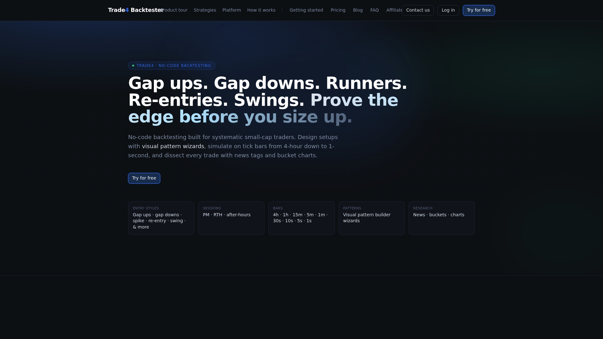
Trade-4 handles the data plumbing so you can focus on the analysis. The platform's visual pattern builder lets you configure IS and OOS date ranges, set slippage and commission assumptions, and run multi-configuration grids from a single interface, all on tick-accurate historical data down to 1-second bars. Each run exports a clean trade log and performance report you can feed directly into your statistical layer. Features like same-day re-entry analytics and news tagging give you the granular OOS breakdowns that matter for small-cap strategies specifically.
If you're ready to move from theory to a working walk-forward experiment, start with Trade-4's no-code backtester and run your first IS/OOS configuration today. The pricing page covers plan tiers and the free trial so you can test the workflow before committing.
This article is general information, not a substitute for advice from a qualified financial advisor. Consult a qualified financial professional about your own circumstances before acting on anything here.
Sources
Start here depending on your goal:
- Machinelearningmastery
- Walk-Forward Backtesting: The Gold Standard for Strategy Validation | ARIA Analyst
- Investment Model Validation — A Guide for Practitioners (CFA Institute)
- Cross-validation: evaluating estimator performance — scikit-learn
- Walk forward optimization — Wikipedia
- A Rigorous Walk-Forward Validation Framework for Market ... — arXiv
Where to run this on Trade4
Apply walk-forward validation on small-cap history without a local tick warehouse:
- Start with the Trade4 getting started guide
- Open the Strategy Builder to set windows, costs, and exits
- Compare history depth and bar size on the pricing page
- Read related research: gap short backtesting and the Trade4 blog