
BLUF: implement half-spread plus a square-root participation impact model as your default fill assumption, then run every strategy through three slippage tiers before you trust an equity curve. This single change closes most of the gap between backtested and live performance, because it captures spread cost, volatility scaling, and the non-linear penalty of trading size. Layer a two-stage location-scale approach (LAD for the median, a scale model for the spread of outcomes) on top, and you get calibrated distributional forecasts instead of a single fragile number.
Run this checklist before you trust any strategy's result:
- Fit baseline / stressed / shock tiers using volatility quantiles, then re-rank your leaderboard under each.
- Cap participation rate per bar and re-check fill assumptions ensuring realistic volume.
- Compare backtest-implied slippage to real TCA or live fills whenever you have them.
- Operationalize the whole loop in a platform like Trade4, which lets small-cap traders run tiered, parameterized backtests without managing local data infrastructure.
Key Takeaways
Accurate performance evaluation depends on modeling slippage as a calibrated distribution across baseline, stressed, and shock tiers rather than a single flat cost assumption.
| Point | Details |
|---|---|
| Default to square-root impact | Use half-spread plus η · σ · sqrt(q/V) as your baseline fill model instead of fixed bps. |
| Calibrate, don't guess | Fit prefactors with LAD for the median and a scale model for residuals, using bucketed, walk-forward data. |
| Test three tiers minimum | Run baseline, stressed, and shock scenarios and check rank correlation between them. |
| Apply slippage inside the loop | Compute fill price after your latency delay, not at signal time, and tag trades with tier metadata. |
| Operationalize with Trade4 | Trade4's no-code backtester lets small-cap traders sweep slippage parameters across historical data without managing local infrastructure. |
Sources and further reading on slippage modeling
Background research included the two-stage LAD and scale calibration project, QuantMedia's latency and fill-model analysis, QuantJourney's non-linear slippage study, Stephen Diehl's spread-estimation code notes, and the MarketMaker blog's practical commentary on cost curves versus constants.
Table of Contents
- What Slippage Modeling Backtest Actually Requires You to Track
- Which Slippage Model Formula Should You Use?
- How Do You Calibrate Slippage Parameters From Real Data?
- Where Does Slippage Get Applied Inside the Backtest Loop?
- How Sensitive Are Your Results to the Slippage Model You Pick?
- How Trade4 Supports This Slippage Modeling Workflow
- The Overlooked Part of Slippage Modeling
- Run Your Slippage Assumptions Through Trade4 Before You Trust Them
What Slippage Modeling Backtest Actually Requires You to Track
A slippage model is only as good as the components it separates. Lump them together and you get a single fudge factor that looks fine in aggregate and fails badly at the trade level. Break slippage into four pieces, and each one maps to a specific number your backtester needs.
- Spread cost. This is the half-spread you cross on entry and exit, expressed in basis points:
(ask - bid) / mid / 2. It's the floor cost every market order pays, even in a perfectly liquid name with zero size. - Market impact, temporary vs. permanent. Temporary impact pushes the price against you while your order executes, then reverts once you're done. Permanent impact is the lasting price shift from information leakage. Backtests typically model the temporary component, as it largely influences the realized fill price on a trade.
- Latency and price drift. Between the moment your signal fires and the moment your order reaches the book, the mid price moves. Model this as a small random walk: drift over the delay window Δt behaves like
σ · sqrt(Δt), where σ is your realized volatility. A 200-millisecond delay in a name with meaningful intraday volatility is not free. - Partial fills and queue effects. Real orders don't always fill in full at one price. A pragmatic way to handle this without full order-book simulation: assign a probabilistic fill rate based on your order size relative to available volume at each price level, and split large orders into simulated child fills across consecutive bars.
Get these four numbers right, and the rest of your slippage model is arithmetic. Get them wrong, and every formula downstream inherits the error.
Which Slippage Model Formula Should You Use?
Model choice depends entirely on how much size you're pushing relative to available liquidity. Four approaches cover almost every situation a small-cap or mid-frequency trader will face.
Fixed basis points is the simplest: apply a flat cost, say 5 to 10 bps, to every fill. It's defensible only under narrow conditions: very low participation rate, highly liquid names, and strategies where position sizing never scales with edge. Outside that box, fixed bps systematically understates costs on your biggest, most impactful trades, which is exactly where the model needs to be most honest.
Half-spread plus impact multiplier is the workhorse for most equity strategies:
P_fill = mid + side · (0.5 · spread + y · σ · (q/V)^δ)
Here side is +1 for buys and −1 for sells, y is your impact prefactor (calibrated, not guessed), σ is realized volatility over the relevant window, q is order size, V is bar or trailing-window volume, and δ controls how impact scales with participation.
Participation-based models formalize the size-scaling piece directly. The square-root law, I(q) = η · σ · sqrt(q/V), is the industry default because concave scaling (δ ≈ 0.5) consistently fits observed impact better than linear scaling. A power-law variant, s(q) = a · q^b, gives you more flexibility to fit b empirically rather than assuming 0.5. Either way, the prefactor (η or a) is where your name-specific and regime-specific calibration actually lives.
AMM/DEX curves follow a different logic entirely. Constant-product pools and similar automated market makers produce slippage that's a direct function of pool depth. Rather than deriving it analytically, query quotes at several order sizes, compute the effective price at each, and fit s(q) = a · q^b empirically. This captures routing effects across pools that a pure formula would miss.
| Model | Best for | Key risk |
|---|---|---|
| Fixed bps | Very liquid names, tiny participation | Understates cost on large or illiquid fills |
| Half-spread + multiplier | General equity strategies, moderate size | Requires calibrated y and δ, not defaults |
| Square-root / power-law | Size-sensitive strategies, growing AUM | Prefactor must be refit as liquidity regimes shift |
| AMM empirical curve | DEX/AMM execution | Needs live quote sampling, not just historical bars |
- Fixed bps is fast to implement but the first model to abandon once size grows.
- The square-root law's exponent near 0.5 is well supported across multiple independent studies of equity impact.
- AMM curves need refreshed quote samples since pool depth changes continuously.
How Do You Calibrate Slippage Parameters From Real Data?
Calibration is where most backtests quietly go wrong. Traders either skip it and hardcode a guessed prefactor, or they overfit a model to a handful of noisy trades. A reproducible calibration workflow avoids both traps.
- Assemble the right data rows. For each historical or simulated order, you need: arrival mid price, realized fill VWAP, parent order size, bar volume at execution time, realized volatility over the relevant window, a spread proxy (from OHLC-based estimators if you lack quote data), exchange identifier, time-of-day bucket, and any relevant event flags (earnings, news, halts).
- Fit the two-stage location-scale model. Stage one uses Least Absolute Deviations (LAD) regression to estimate the conditional median slippage,
μ̂(x), given your features. Stage two regresses the absolute residuals from stage one to estimate the scale,b̂(x). This two-step structure fits microstructure data well because trade cost residuals behave closer to a Laplace distribution than a normal one, with fat tails driven by occasional bad fills. - Stabilize the fit with bucket medians. Single-order slippage is dominated by noise. Grouping trades into buckets by size, volatility regime, or time of day and taking medians within each bucket produces far more stable level estimates than trying to fit every individual trade point.
- Cross-validate with TimeSeriesSplit, never a random shuffle. Slippage has serial structure. Use walk-forward validation and be ruthless about excluding any feature that wasn't actually available at decision time. Refit the whole model on a quarterly cadence, since liquidity regimes drift.
- Extract η, y, and δ through regression or non-linear least squares, and bootstrap confidence intervals around them. A point estimate for your impact prefactor without an uncertainty band tells you almost nothing about how much to trust a backtest run on it.
Published results on this exact two-stage approach show something that surprises a lot of engineers the first time they see it: out-of-sample R² for the point forecast is often low, because microstructure noise genuinely dominates individual trade outcomes. What matters operationally is coverage. A well-calibrated model targeting 90% prediction intervals should land close to that in practice, which is usable even when the point estimate itself explains relatively little variance.
Pro Tip: Don't discard a slippage model because its R² looks unimpressive. Check interval coverage instead. A model that nails 90% coverage on out-of-sample data is doing its actual job, which is bounding your risk, not predicting every trade's exact cost. For feature engineering on relative spread and liquidity proxies, a tool like TP Scanner can help surface the microstructure inputs your calibration needs before you commit to a parameter set.
Where Does Slippage Get Applied Inside the Backtest Loop?
The fill formula needs a home in your backtest architecture, and where you put it changes everything downstream. The canonical expression:
P_fill = M_(t+Δt) + side · (0.5 · S_(t+Δt) + I(q)) + ϵ
Here M_(t+Δt) is the mid price after your latency delay, S_(t+Δt) is the spread at that same future point, I(q) is your impact function, and ϵ is residual noise drawn from your calibrated scale model. Notice the price and spread are both evaluated after the delay, not at decision time. That single detail is where a lot of backtests quietly cheat.
The recipe, step by step:
- Signal fires at time
t. Freeze all features computable from information available att, nothing later. - Compute the delay window
Δtand project the mid and spread forward using your drift model. - Feed order size, volatility, and volume into your calibrated model to get a predicted slippage distribution, not just a point.
- Either sample from that distribution (for Monte Carlo style runs) or apply the median for a deterministic single-path backtest, tagging the run with which choice you made.
- Apply the resulting fill price to the executed quantity only, updating P&L and inventory. If the order only partially fills, split it into child fills across subsequent bars and repeat the process for the remainder.
- Log the slippage tier and model version used on every trade, so results can be traced back to the exact assumption set that produced them.
Treating slippage as a downstream adjustment to a "clean" backtest is the single most common architectural mistake in this workflow. Slippage assumptions belong inside the strategy definition itself, tested alongside your signal logic, not bolted on after the fact as a tax on returns.
Partial fill handling deserves its own attention. A probabilistic fill rate tied to your order's participation relative to bar volume, combined with explicit child-order slicing for anything resembling TWAP or VWAP execution, keeps orphaned partial fills from silently vanishing out of your performance metrics. Fix your random seeds for reproducibility, vectorize the prediction step if you're running large batches of scenarios, and tag every trade with its slippage tier metadata so you can slice results later without rerunning the whole backtest.
How Sensitive Are Your Results to the Slippage Model You Pick?
This is the question most backtests never answer, and it's the one that matters most. A strategy that looks profitable under one slippage assumption can lose money under another, even when both assumptions look reasonable on paper.
Start by defining three tiers, typically based on volatility quantiles: baseline (normal market conditions), stressed (elevated volatility, wider spreads), and shock (crisis-level conditions with thin liquidity). Apply tier-specific multipliers to your impact prefactor rather than building three separate models from scratch.
Then run a parameter sweep. Vary η and δ across a realistic range and measure how much your strategy leaderboard reshuffles. Rank correlation, using something like Kendall's tau, between your baseline model's rankings and a stressed model's rankings tells you directly how fragile your winners are.
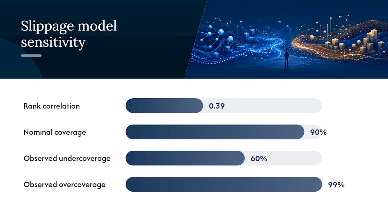
- One documented comparison of cost models found a low rank correlation between two reasonable slippage assumptions, indicating the model choice alone can reorder which strategies look best.
- Check prediction interval coverage on held-out data before trusting any tier's output; a 90% nominal interval should land close to 90% actual coverage, not 60% or 99%.
- Compare backtest-implied slippage against live TCA whenever you have real fills to check against, and treat persistent gaps as a signal to refit, not a rounding error.
- Publish which slippage tier produced each equity curve, and version your slippage model alongside your strategy code so past results stay reproducible.
That 0.39 correlation figure is worth sitting with. It means two defensible cost models can send you toward almost opposite conclusions about which strategy to trade live.
How Trade4 Supports This Slippage Modeling Workflow
Running this calibration-to-backtest loop by hand across dozens of strategies gets tedious fast, which is exactly the gap Trade4 was built to close for small-cap traders. The no-code backtester lets you configure entry, exit, and risk filters visually, then apply cost assumptions across tick-to-one-minute historical data without writing custom simulation code.
- Visual pattern builders let you encode the fill logic and participation caps described above without touching Python.
- News tagging and analyzer features flag event-driven bars, which matters since impact and spread both widen around catalysts.
- Same-day re-entry analytics show how slippage tiers affect strategies that re-enter positions intraday, a case where naive fixed-bps assumptions fail hardest.
Pro Tip: Use Trade4's job queue and multi-run buckets to sweep η and δ across a grid of values overnight, then compare the resulting leaderboards the next morning instead of babysitting each run. For a concrete walkthrough of setting up a strategy with these filters, the guide on backtesting gap short strategies on small caps shows the same building blocks in action.
The Overlooked Part of Slippage Modeling
Most guides to slippage modeling spend their energy on the impact formula and treat calibration as an afterthought. That's backward. The square-root law with δ ≈ 0.5 is well established and not really in dispute. What actually separates a useful slippage model from a decorative one is whether the prefactor was fit on real, bucketed, walk-forward-validated data, or just borrowed from a paper and left there.
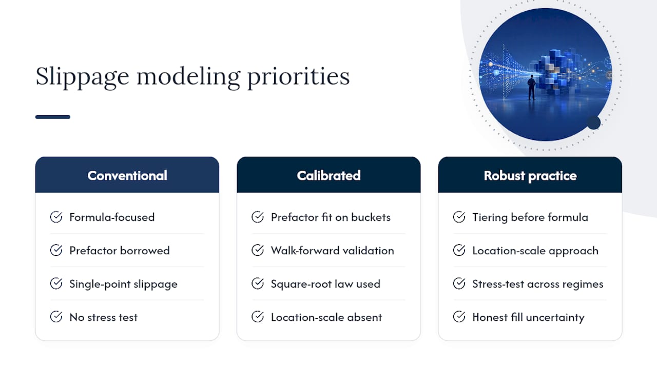
The other place conventional advice falls short is treating slippage as a single number to report alongside an equity curve. A point estimate hides exactly the risk you're trying to measure. The two-stage location-scale approach is more work to set up, but it gives you something a flat assumption never will: an honest sense of how wrong your fill estimate could be on any given trade, not just on average.
If you take one thing from this, prioritize the tiering before the formula. A perfectly calibrated impact model tested only under baseline conditions will still blindside you the first time volatility spikes and your rank correlation between tiers collapses. Build the stress test first, refine the formula second.
— Romans
Run Your Slippage Assumptions Through Trade4 Before You Trust Them
Trade-4 gives small-cap and algorithmic traders a direct way to turn everything above into a working backtest, without standing up local infrastructure to manage tick data or run custom Monte Carlo loops. Instead of hand-coding the fill formula and slicing partial orders in a script, you configure entry, exit, and cost assumptions visually and let the platform run tiered scenarios across historical data down to one-second granularity.

That matters most for the exact fragility problem this article covers: a strategy that looks strong under one slippage assumption can fall apart under another, and Trade4's granular bar data plus bucketed performance analysis let you see that reordering before you risk real capital on it. Same-day re-entry analytics and news tagging cover the two conditions where naive fixed-bps assumptions break down fastest. If you're ready to test your own strategy across baseline, stressed, and shock assumptions, walk through the getting started guide and run your first tiered backtest this week.